From Silicon Labs: "Timing 101 #9: The Case of the Discrepant Scope Measurements"

Introduction

In English, we often use the expression “comparing apples to apples” to mean we are making a fair comparison between similar things. On the other hand, if we are “comparing apples to oranges” then we mean the opposite.

Sometimes, despite our best efforts, our lab measurements may yield an instance of “apples to bruised apples”. In this month’s post, I will provide a relatively common example in The Case of the Discrepant Scope Measurements.

The original case

Years ago, I was supporting an oscillator customer and we were having correlation issues, i.e. his measurements versus mine. His period jitter measurements were just not making any sense compared to the spec and to the part’s typical performance.

I knew enough to make sure that we had similar boards, cables, terminations, test equipment, and were at least attempting the same measurements. We even had very similar oscilloscopes. I was starting to wonder if there really could be something amiss with his device when I asked him to send me a scope shot of his waveform. Bingo! His waveform was a fraction of the size of mine and I knew that was most likely the source of the discrepancy.

Example Lab Measurements

To illustrate the issue I took a nominal 2.5V LVDS 100 MHz output clock and measured it with a good quality 1 GHz DSO or Digital Storage Oscilloscope that supports measurements statistics (the higher bandwidth scopes were all tied up and 1 GHz is sufficient here.) I took each measurement a little over 10K times, varying only the vertical scale, and tabulated the key results below. Note that I record the measurements below in decreasing vertical scale. The smaller the vertical scale, the larger the displayed waveform.

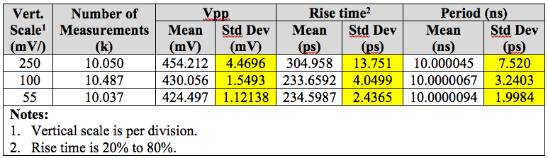
The most notable observation is that the standard deviation of all of the measurements decreased with vertical scale. The smaller the vertical scale, and the larger the displayed waveform, the more accurate the measurements.

One Man’s Noise is Another Man’s Signal …

I am particularly interested in the period jitter, which is the standard deviation of the period measurements. If we plot period jitter versus vertical scale from the table values we obtain the following linear plot.

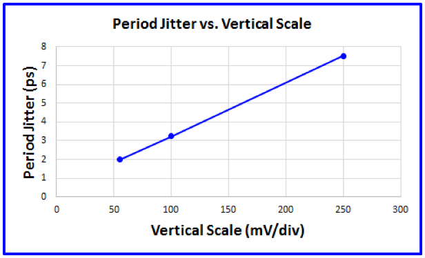
The measured period jitter versus the scales sampled appears linear. Further, there was no deflection at the smaller values suggesting we were not approaching a measurement “floor”.

Before discussing why the measurements turned out the way they did, let us briefly review the screen caps for each scale selection and why we might use them.

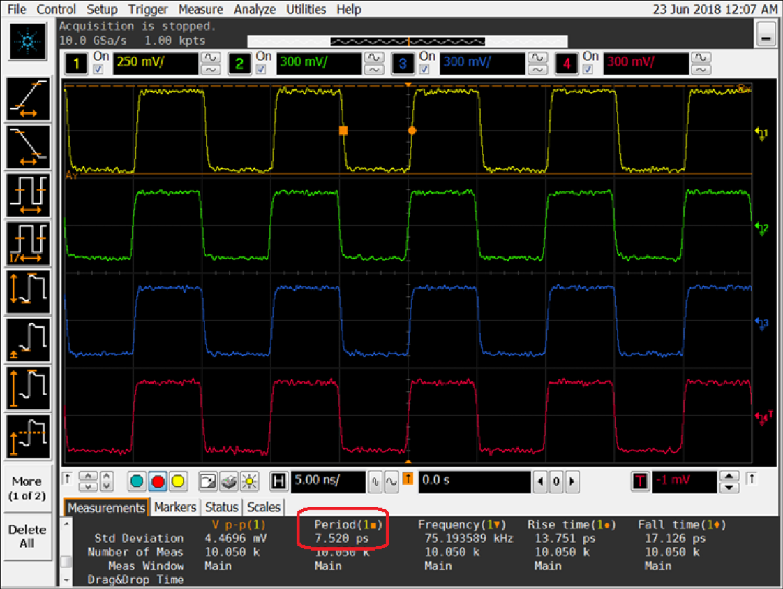
The 250 mV/div selection

This is the smallest displayed waveform selection of the three instances. You run in to this type of scaling when attempting to measure several waveforms simultaneously, for example when comparing relative clock skew. The standard deviation of the period measurements, i.e. the period jitter, was 7.5 ps.

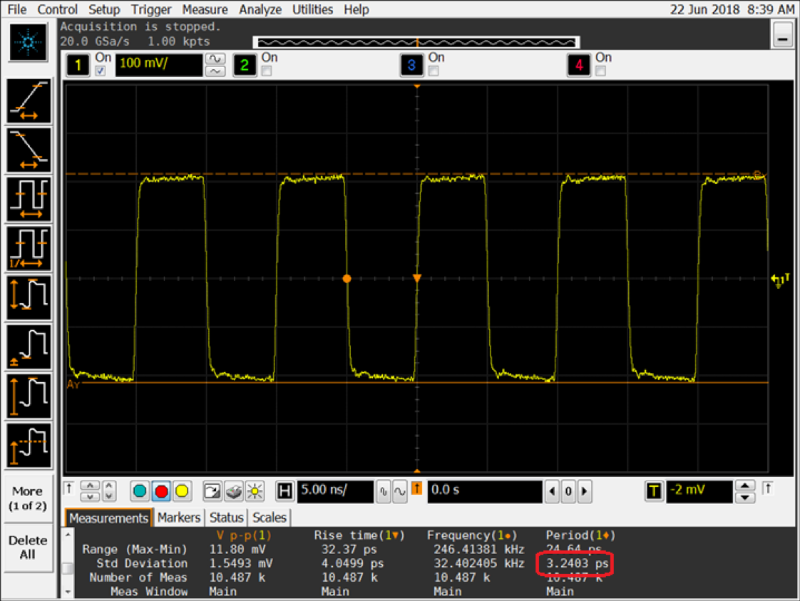
The 100 mV/div selection

This is the most common selection as it is the default or auto scale selection for this particular scope when measuring a single waveform. The period jitter dropped by more than half to 3.2 ps. Great for browsing but as it turns out, still not optimum.

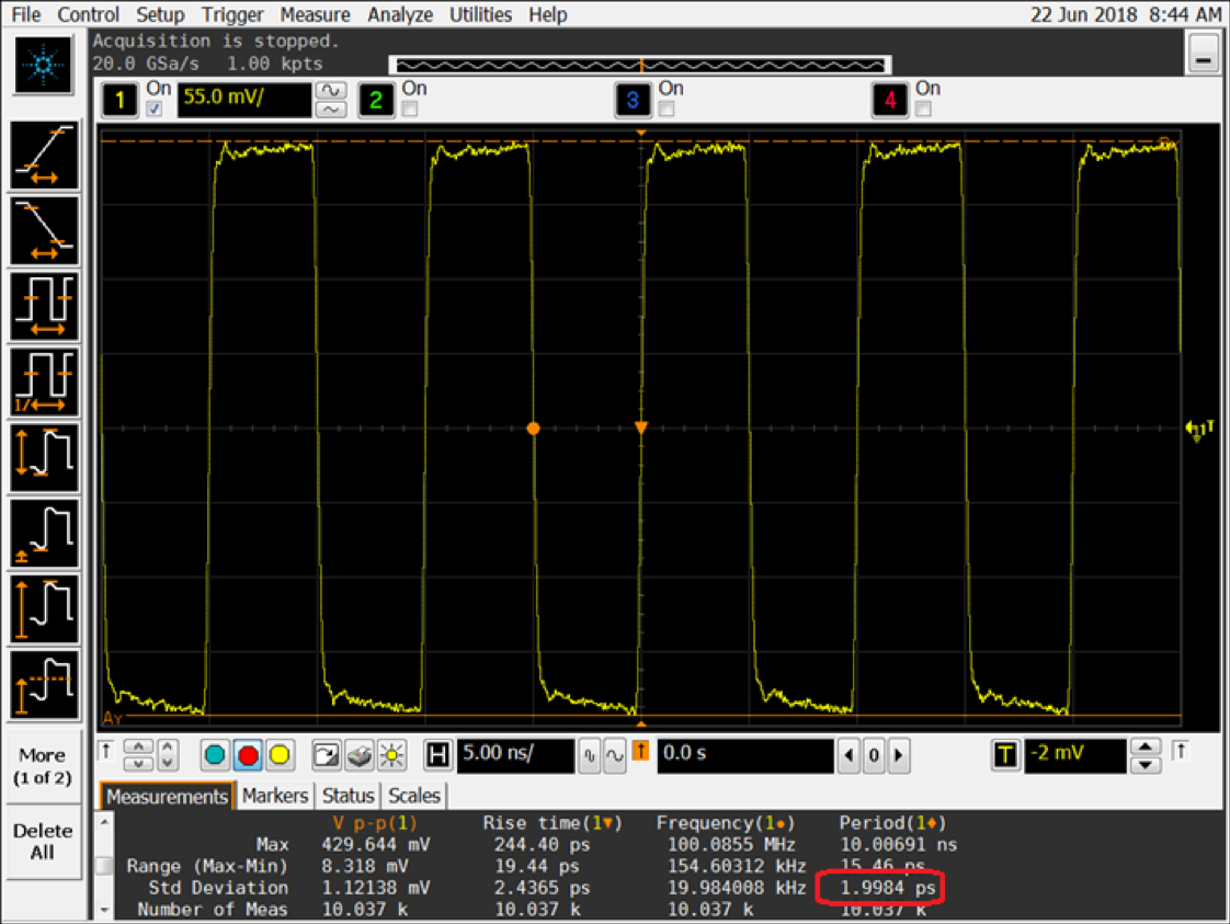
The 55 mV/div selection

This final selection maximizes the displayed waveform on the scope without clipping. The period jitter dropped to about 2 ps. 

An Explanation

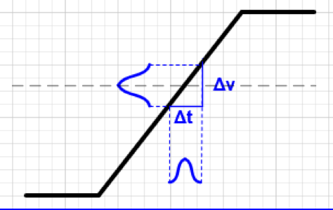
I purposely did not make any sampling or time scale changes in these measurements in order to eliminate that aspect as a variable. The only change is in vertical scaling which impacts voltage noise. Voltage noise translates to timing noise via slew rate, i.e. the ratio of delta voltage over delta time, as illustrated in the exaggerated figure below. The blue Gaussian curves are intended to suggest normal noise distributions about the decision threshold.

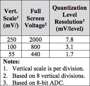
The DSO is a digital scope with a sampling ADC in the front end of the signal chain. The voltage noise will therefore be due to the DUT and the DSO’s ADC quantization noise. This particular scope’s ADC is nominally 8 bits. (The actual ENOB or Effective Number Of Bits may be lower but the principle is the same.)

An 8-bit ADC has 256 unique codes or quantization levels. Therefore, we can compare the nominal quantization levels as follows. There is a significant reduction in quantization noise as we decrease vertical scaling.

The ADC’s 8 bits are employed across the entire vertical display of the oscilloscope so anything less will use fewer bits and result in more quantization noise. This in turn yields more timing uncertainty. It is for this reason that oscilloscope manufacturers often recommend that users maximize the waveform on the screen for most accurate measurements. Doing so without clipping the waveform is the most conservative approach but check with your particular scope vendor.

Conclusion

I hope you have enjoyed this Timing 101 article. Comparing digital scope measurements, which don’t have similar vertical resolution, can result in comparing “apples to bruised apples”.

As always, if you have topic suggestions, or there are questions you would like answered, appropriate for this blog, please send them to kevin.smith@silabs.com with the words Timing 101 in the subject line. I will give them consideration and see if I can fit them in. Thanks for reading. Keep calm and clock on.

Cheers,

Kevin

Source: https://www.silabs.com/community/blog.entry.html/2018/06/29/timing_101_9_thec-TDnn