From Silicon Labs: "Timing 101 #8: The Case of the Cycle-to-Cycle Jitter Rule of Thumb"

Introduction

In this post, The Case of the Cycle-to-Cycle Jitter Rule of Thumb, I will review a rule of thumb that can be used for estimating the RMS cycle-to-cycle jitter if all you have available is the RMS period jitter. The reason I’m doing so this month is that a couple of colleagues of mine recently asked me to reconcile a particular Timing Knowledge Base article versus one of our app notes . I first observed this rule of thumb in the lab and subsequently learned more about it.

What’s the Rule of Thumb?

It’s real simple. If the period jitter distribution is Gaussian or normal, then the cycle-to-cycle jitter can be estimated from the period jitter as follows:

Jcc (RMS) = sqrt(3) * Jper (RMS)

I first recorded this in a Timing Knowledge Base article Estimating RMS Cycle to Cycle Jitter from RMS Period Jitter. I wrote at the time the following statement:

The sqrt(3) factor arises from the definitions of period jitter and cycle-to-cycle jitter in terms of the timing jitter of each clock edge versus a reference clock.

I will spend a little bit more time on this thought today and attack the problem from several different angles.

What’s the Question?

In our application note, A Primer On Jitter, Jitter Measurement and Phase-Locked Loops, the figure below shows the following slopes for post-processing phase noise into timing jitter metrics. Period jitter and cycle-to-cycle jitter are shown as high pass filters with 20 dBc/dec and 40dB/dec slopes, respectively. This is correct and a useful illustration to keep in mind.

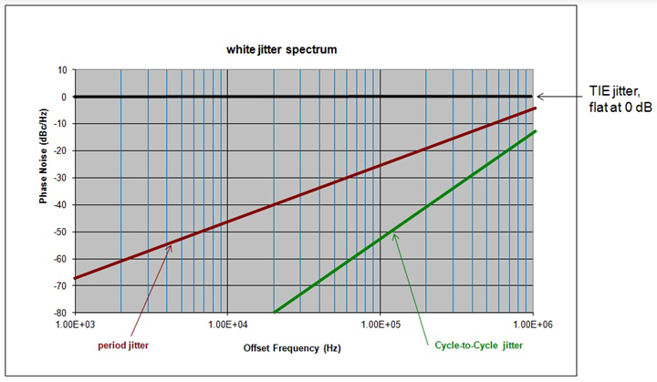
The question is how can RMS cycle-to-cycle jitter be larger than RMS period jitter, per the sqrt(3) rule, and the cycle-to-cycle jitter filter have a steeper slope? The answer is that it’s not just the slope that determines the end result. More on that later.

Some Terminology

Before proceeding, here are a couple of definitions adapted from AN279: Estimating Period Jitter from Phase Noise.

• Cycle-to-cycle jitter - The short-term variation in clock period between adjacent clock cycles. This jitter measure, abbreviated here as JCC, may be specified as either an RMS or peak-to-peak quantity.
• Period jitter - The short-term variation in clock period over all measured clock cycles, compared to the average clock period. This jitter measure, abbreviated here as JPER, may be specified as either an RMS or peak-to-peak quantity.

The distinction between these time domain jitter measurements is important, hence the italicized terms above. (By the way, you can find old examples in the academic and trade literature where these terms may mean different things, so always double-check the context). The terms here are as used presently and in standards such as JEDEC Standard No. 65B, “Definition of Skew Specifications for Standard Logic Devices”.

Example Lab Measurement

First, the following example lab measurement comes straight from the KB article. The annotated image has been made more compact for convenience.

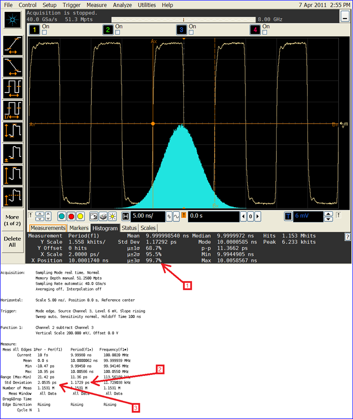
There are three items called out on the screen capture.

1. The period distribution after 1 million cycles appears Gaussian and comes very close to meeting the 68-95-99.7 % rule for ±1, ±2, and ± 3 standard deviations respectively.
2. The measured RMS period jitter is the standard deviation of the period jitter distribution or about 1.17 ps.  We can therefore estimate the RMS cycle to cycle jitter as sqrt(3) * 1.17 ps or 2.03 ps.
3. The actual measured cycle to cycle jitter is 2.05 ps which is reasonably close to the estimate.

Example Excel Demonstration

You can also demonstrate this rule in Excel simulations. Exploring the effect, I generated a spreadsheet where I took an ideal clock edge and then jittered the edges by taking random samples from a Gaussian distribution. I then took the period measurements, and the cycle to cycle measurements, over five trials each for 30 edges, and 100 edges with the clock edges representing a jittery 100 MHz clock. Note that since the cycle-to-cycle jitter results are signed, i.e. positive or negative, we should expect the standard deviation of these quantities to be larger, all else being equal. The 100 edges trials were usually much closer to the sqrt(3) rule than the 30 edges trials but you could still see the general effect even over just 30 edges.

If you are interested in playing with it, the spreadsheet is attached as CCJ_ROT_Demonstrator.xlsx. 

An Explanation

So how does this rule of thumb arise? As mentioned previously, I first observed this in the lab years ago and learned I could count on it. Yet, I have seen little written about this. Eventually I ran across Statek Technical Note 35, An overview of oscillator jitter. The explanation below is a somewhat simplified and modified version of that derivation where the quantities are expected values for a “large” time series (recall my comments about 100 edges converging to the rule better than 30 edges.)

Let the variable below represent the variance of a single edge’s timing jitter, i.e. the difference in time of a jittery edge versus an ideal edge.

Every period measured then is the difference between 2 successive edge values, where each edge jitter has variance s2j. Period jitter is sometimes referred to as the first difference of the timing jitter. Since cycle-to-cycle jitter is the difference between adjacent periods it can be referred to as the second difference of the timing jitter.

If each edge’s jitter is independent then the variance of the period jitter can be written as

This is just what we would expect per the Variance Sum Law. You can see an example here, which states that for independent (uncorrelated) variables:

However, we can’t calculate cycle-cycle jitter quite as easily since in every cycle-to-cycle measurement we use one “interior” clock edge twice and therefore we must account for this. Instead we write:

Since each edge’s jitter is assumed to be independent and have the same statistical properties we can drop the cross correlation terms and write: 

The ratio of the variances is therefore

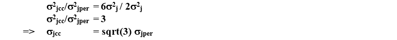
This is an interesting and unexpected result, at least to me :)  

Post-Processing Phase Noise

AN279: Estimating Period Jitter from Phase Noise describes how one can estimate period jitter from phase noise based on applying a 4[sin(pi*f*tau)]^2 weighting factor to the phase noise integration. The weighting factor is predominately a +20 dB/dec high pass filter until reaching a peak at the half-carrier frequency.

It turns out that you can use a similar approach to calculating cycle-to-cycle jitter. This requires applying a {4[sin(pi*f*tau)]^2}^2 or 16[sin(pi*f*tau)]^4 weighting factor which is predominately a +40 dB/dec high pass filter until reaching a peak at the half-carrier frequency.  This is exactly what AN687 refers to.

So how can a sharper HPF skirt integrate such that cycle-to-cycle jitter is larger than the period jitter and the sqrt(3) rule applies?

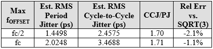
I had to dig up my old Matlab program which I used when writing that app note. Fortunately, I still had the file and the original data. I then ran a modified version of the program and compared the results for max fOFFSET where the phase noise dataset is extended and truncated at both fc/2 and fc. The answer is that while the cycle-to-cycle HPF skirt is steeper the maximum is also higher. See the plots below. The blue wide trace is the period jitter weighted (filtered) phase noise and the red wide trace is the cycle-to-cycle jitter weighted phase noise.  It’s the larger far offset phase noise contributions that make the difference.

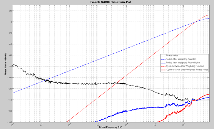
The original data was for a 160 MHz CMOS oscillator which had a scope measured period jitter at the time of about 2 ps. To be conservative, it was for that reason that I often ran the integration further out than fc/2. Scopes are lower noise now and it would be interesting to go find the original device under test and measure it on a better instrument. My main interest here is to see if the sqrt(3) relationship holds true. As you can see, the rule of thumb holds up in both cases.

Conclusion

Well I hope you have enjoyed this Timing 101 article. The sqrt (3) rule of thumb for cycle-to-cycle jitter holds up well in the lab, in Excel spreadsheet simulations, and when post-processing phase noise.

As always, if you have topic suggestions, or there are questions you would like answered, appropriate for this blog, please send them to kevin.smith@silabs.com with the words Timing 101 in the subject line.  I will give them consideration and see if I can fit them in. Thanks for reading. Keep calm and clock on.

Cheers,

Kevin

Source: https://www.silabs.com/community/blog.entry.html/2018/05/23/timing_101_8_thec-CaxZ